
xG has become the most-used ‘advanced’ metric in football analysis. Everybody seems to have an xG model nowadays, yet all are different. This begs the question, how good are they? Last year I tried to answer this question by evaluating a bunch of xG models. It got quite some attention and so I felt it would only be right to replicate the test this season.
The results however, were different than expected. These surprising results might hint at a flaw in most xG models that are used at the moment. I will go into this further in the second paragraph, but first I’ll show the results of the contest!
The contest
Let’s first introduce all contestants, and also the additional benchmarks we’ll be testing:

Methodologies (if online) can be found in the appendix1. Apart from the new contestants, I also decided to include Paul Riley’s model from his blog ‘An xG model for everyone in 20 minutes’ to see how it performed. For an explanation of how the ‘perfect’ model is created, please read my blog from last year. For the ‘All shots equal’ model, I use a value of 0.095 for every shot, as proposed in a Deadspin article a while back.
We’ll be testing the models by calculating the RMSEP of the xG values and the actual amount of goals. RMSEP is a measure used to evaluate the differences between predictions (xG) and outcome (goals). Just like last year, this measure will be used since it allows for comparison with the ‘perfect model’. Penalties and own goals are excluded. For a more exact explanation of methodology, please refer to my blog last year.
Without further ado here are this year’s results:
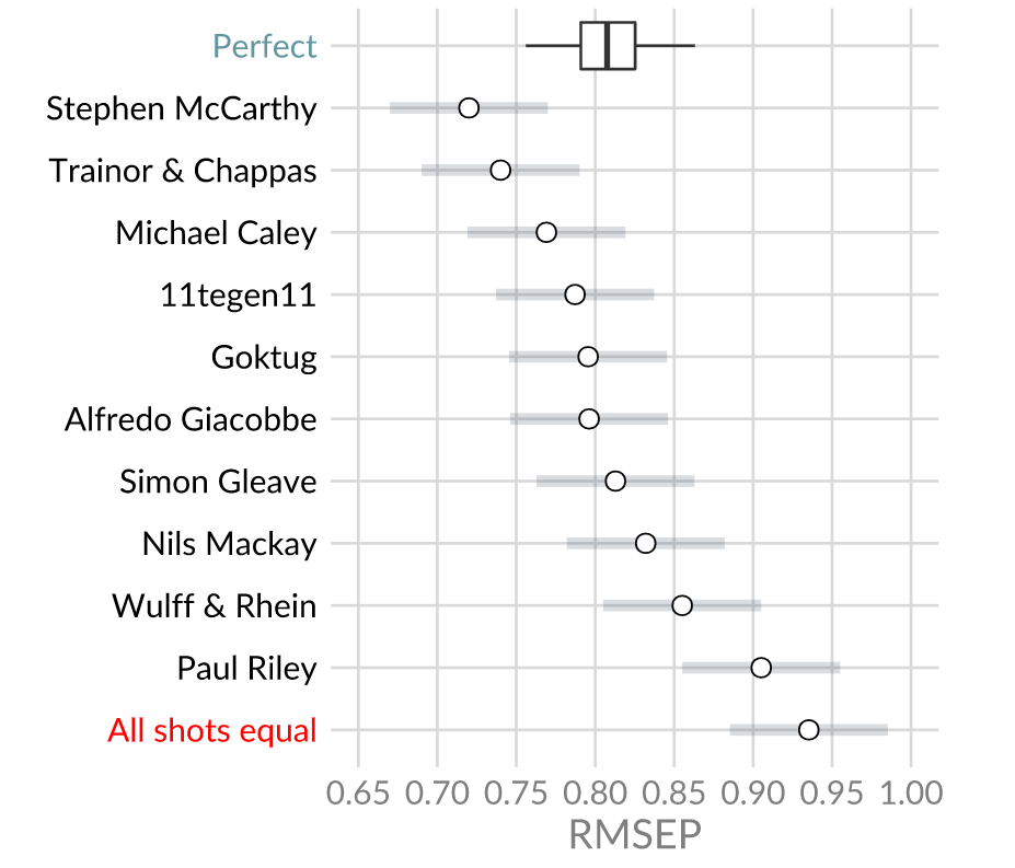
The winner is:… Stephen McCarthy!
Newcomers Colin Trainor and Constantinos Chappas take 2nd place. Winner and runner-up from last year Michael Caley and 11tegen11 finish 3th and 4th respectively. Also, all models perform better than the ‘all shots equal’ benchmark. Even the relatively simple model proposed by Paul Riley outperforms the benchmark by quite some difference.
You might’ve noticed something funny though…
How come most of the models perform better than the perfect model does on average? Some models are even outside the 95%-confidence interval. That means the possibility that this season is some sort of outlier is very small. What is going on here?
There are two possible explanations. The first is that the perfect model might not be accurate. The perfect model is based on my xG values. That means that if it’s calculated for a different distribution of xG values, the RSMEP may differ. I tried to test this by taking a few similar looking distributions (sampled from my xG values, and exponential) to see how that would change the average RMSEP. As it turned out, not much changed. Therefore I don’t think this (fully) explains these weird results.
The second explanation seems much more plausible to me. It revolves around OPTA’s Big Chance metric.
The Big Chance Dilemma
A ‘Big Chance’ is a variable that is recorded by OPTA. The idea behind it is that it will be a 1 when a shot is a big chance, and a 0 otherwise. OPTA coders decide after a shot whether it was a ‘Big Chance’ or not, and double check these decisions afterwards.
Most xG models use this variable as it can be used as a proxy for defensive pressure. Since there’s no public tracking data available for most leagues, this seems like a good way to fill the gap of missing information. For instance, ‘Big Chance’ might be able to take into account how many players there are between the ball and the goal.
Sounds good right? Well…
It is very likely that OPTA coders fall prey to something called ‘outcome bias’. Freely transcribed from Wikipedia: “Outcome bias is an error made in evaluating the quality of a [chance] when the outcome of that [chance] is already known.” Basically, when a player converts a chance, it will be more likely for coders to note it as a ‘Big Chance’. On the other hand, when a player messes up, it might in retrospect look like a more difficult chance, and the ‘Big Chance’ label might not be given.
This means that the ‘Big Chance’ metric indirectly includes post-shot information. It can be (roughly) compared to making a model that uses ‘shots on target’ only. Such a model will always perform better than an ‘all shots’ model in the above contest, as they will simply have more information. This makes it impossible to accurately compare models in the way I did above. Some models might use the ‘Big Chance’ metric more, which will give them a bigger advantage. Others might barely use it and end up at the bottom. When looking at the results from earlier this becomes clear:
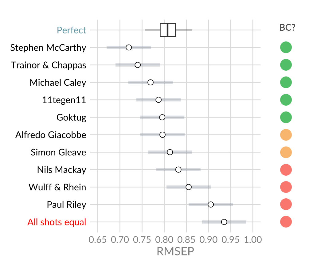
Model with a green circle used OPTA’s Big Chance metric. Models with an orange circle used a Big Chance variable but not the one from OPTA. Models with a red circle didn’t use a Big Chance variable at all. The difference in ranking is easily seen.
Apart from putting a huge ‘?’ next to the contest results, it is also questionable if we should want to use the ‘Big Chance’ metric in our models at all.
- Descriptive vs. predictive
xG models can be made for several purposes. However, as far as I know, most make them to get a better view of underlying performance. We all know goals are surrounded by a cloud of randomness and xG is a great way to see through that somewhat. That way we can judge player/team performance better. For instance we could say:
- “Hey the results are bad, but it’s plausible that, seen their good underlying performance, they will improve in the future.”
- “Hey the results are bad, and so is the underlying performance, they should change something.”
In both cases you make a judgement on team performance based on your projection of how it will be in the future. I feel most of xG figures are used for this purpose.
That being said, it is questionable if the Big Chance metric improves this process. It correlates with goals very well, and thus your xG model will be more apt to predict if a shot was a goal. However, the predictive performance of it might not become better. Taking post shot information might mean overfitting on outcome, rather than accurately measuring process. Whether this is true or not is to be seen, but the fact that I haven’t seen someone write about this yet tells me most people don’t even consider this. (Out of the methodologies I’ve seen only Michael Caley acknowledge this issue and try to correct for it.)
- Dependency
The possible impact of the Big Chance variable on predicted xG values has been shown by Jan Mullenberg in a blog he wrote about xG models:
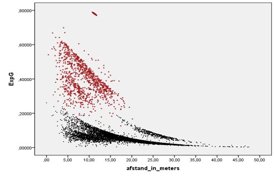
What you see above is the predicted xG on the y-axis, and the distance to the goal on the x-axis. The red dots are shots classified as a Big Chance, whereas black dots are not. It is baffling to see that the impact is so big, that a ‘bad’ Big Chance almost always has a higher xG value than a ‘good’ non-Big Chance. An example2 of this impact in real life:
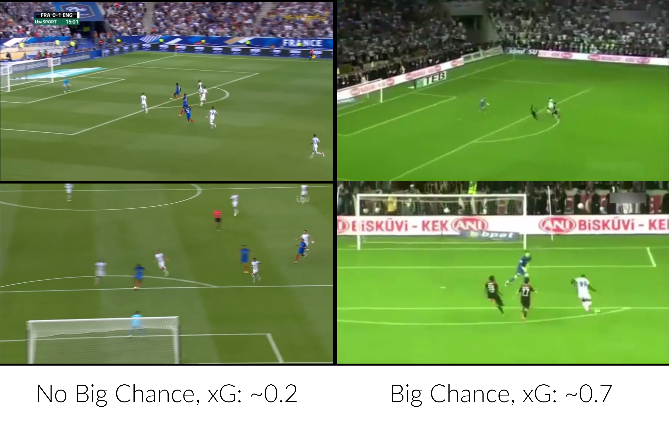
I’m not saying the left chance is definitely a better chance than the right one. However it’s safe to say the difference should not be anywhere close to 0.5. To have a model rely on one subjective variable this much can’t be good.
- Inconsistency
[NOTE: From reliable sources I’ve heard that the following paragraph only applies to data that has been scraped. Opta does Big Chances for all matches they keep track of. Therefore the following paragraph only applies to public models, and not to models built on an actual Opta feed.]
Going through my Twitter timeline, I often encounter xG maps of matches I recently watched. Just last week, I noticed something weird. I’d watched the international friendly between The Netherlands and Côte d’Ivoire, in which the Netherlands won 5-0. When looking at the xG plot from @11tegen11, I noticed the xG score for some chances were much lower than I’d expected. After enquiring with Sander it turned out none of the shots from that match were noted as a ‘Big Chance’. This was surprising, as that meant that for instance this shot from Janssen was not considered a ‘Big Chance’.

Actually, none of the shots in this match was valued as a ‘Big Chance’, indicating that OPTA might only use the ‘Big Chance’ variable for certain leagues/matches. The problem here is, nobody knows which matches! Using an xG model fitted on ‘Big Chances’ for matches like this will make the total xG score much, much, lower than what it should’ve been. This will hurt predictive power, but also the descriptive part of xG. You might for instance look at Janssen’s performance in the national team and conclude that his xG numbers were weak, even though they should’ve been much higher.
I hope you all agree these are some serious issues surrounding xG models, that I feel aren’t given enough attention. What this is not is a call to stop using the Big Chance variable. What this is, is call to all modelers out there to reevaluate your choices. The Big Chance might seem like a great way to model defensive pressure, but its flaws and the errors it creates might not be worth it.
Appendix:
1 Methodologies:
Paul Riley: An xG model for everyone in 20 minutes
2 The left example is from the international friendly between England and France, shot by Dembele around the 15 minute mark. The right example is from Gaziantepspor – Besiktas, from the Turkish Süper Lig, somewhere between the 0-4 and the final whistle.