How NOT to evaluate your xG model

Expected goals is a complex metric. Not only because it is difficult to calculate, but mostly because the models are very hard to evaluate. This is something I realized after recently creating my own Expected Goals (xG) model. (For those who are unaware what xG means; it’s a metric describing the probability a certain shot will end up being a goal. The simplest example for this is a penalty, which has an xG of about 0.75. In other words, about 3 out of 4 penalties are scored.) I soon realized it is very hard to determine how good my model really was, as I had nothing to compare it with.

Therefore I first set out on making a benchmark. In this case that benchmark would be a perfect xG model, so it is possible to ask yourself: how close is my model to being perfect? *(What does a ‘perfect’ xG even mean? I discuss this in the appendix since it is quite technical.)

How can you possibly have a perfect xG model?

I don’t. If I would I probably wouldn’t even have to write this article. It is however fairly simple to find out how a perfect model would perform. I might not know the exact xG values for all shots during this BPL season, but let’s assume I do know them for this BPL season in an alternate universe (stick with me). Let’s just for now assume that the xG values I calculated for this BPL season were actually 100% correct (which they are definitely not). The only thing we miss now are actual results in this ‘second universe’, so to gather these all I had to do was simulate all matches once using the ‘perfect’ xG values. This is also known as a Monte Carlo simulation. This gives one possible outcome of all matches. Let’s look at a 4-shot example:

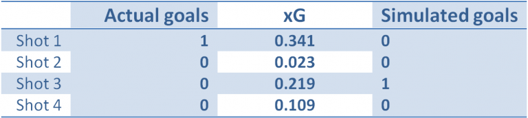
At the left we can see that in reality, out of these shots only shot 1 was scored. Next to that we can see the xG value my model assigned to those shots. Simulating these xG values gave the results on the right. These simulated goals now have the xG values as their true underlying probabilities. In other words, these xG values are ‘perfect’ and the ‘simulated goals’ on the right is one of the possible outcomes.

Whatever measure we are going use, we can always check how a ‘perfect’ model would perform to compare. In the rest of this article, I will use this method as a benchmark.

R-squared is really, really not ok

When checking around the web what methods were used, I was surprised to see that R² was the most common way of evaluating whether an xG model was any good. In most cases I would see a plot similar to this:

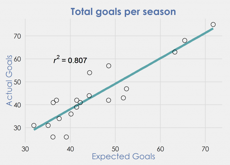
What we see here is the amount of goals all 20 teams in the 2014/2015 Premier League scored, and the sum of the Expected Goals a model of mine assigned to all shots taken by that team. Next I applied a linear regression which gave a R² of 0.807. This sounds great!

But it isn’t. For several reasons:

1. Information loss
   By summing all the xG values over a season, we lost a huge amount of data. We started with around 10000 points but reduced it to 20. Furthermore, this only gives us a sample size of 20, which is way too small.

2. Is 0.807 even good?
   How good is this R² figure really? Apart from the fact that the small sample size probably means that the value relies heavily on variation, it is also not as good as it sounds. If we simply count the shots a team attempts in a season and plot it against the goals scored, in this specific example you’ll get an R² of 0.712! Over large samples like we use in this example, the xG per shot tends to be pretty similar for all teams, meaning the xG values you calculated won’t improve your results by much. Even more shockingly, a single simulation of the ‘perfect’ model gave a R² of 0.755, which is lower than what our model achieved. Obviously over a larger sample of shots it will outperform my xG model, but the fact that it doesn’t here shows how unreliable these numbers are. The variance over such a small sample size appears to be so big, that we really can’t say anything useful about this R² value.

3. It’s theoretically wrong
   R² measures how much variation of the response variable (actual goals) is explained by the decision variable (xG). To do this it finds a linear function that is the best fit. The line in the above example is:

Actual goals = -6.18 + 1.11 * xG

This is NOT what we try to model when we create xG. The idea behind xG is that 1 xG is worth exactly 1 actual goal, which is not what is assumed by the linear regression method. For example, using the above formula we would expect to score 38 goals when we score 40 xG. This is clearly not what we aim to measure when using an xG model.

Go on then smartass, what metric should we use?

I have to admit that although I know R² is wrong, I’m not sure what the best way is to evaluate xG models. Personally I believe a good way to evaluate an xG model is by looking at smaller samples than entire seasons. One could for instance look at single match totals of xG values and actual outcomes. That will make the influence of individual xG estimations much bigger, while single matches usually are the smallest sample in which we actively look at xG.

In an upcoming blog I will explain this method. Furthermore I will evaluate a set of xG models from i.a. Michael Caley, SciSports, @SteMc74, myself and more, using this method. Then we’ll finally know how close we are to a perfect xG model and which one is closest. If you want to participate with your own xG model please contact me on Twitter (@NilsMackay).

*Appendix (What is a perfect xG value?)

Since xG attempts to predict whether a shot ends up in the goal or not, one might say that a perfect xG model takes into account all possible variables. It would take into account things like: wind speed, wind direction, keeper positioning, the keeper’s reaction time, the way the ball is hit etc. However, such a model would perfectly predict whether a shot will become a goal or not and therefore only return values of 1 and 0. In other words for every shot it would say either: “Yes, this shot will become a goal” or “No, this shot will not become a goal”. Such a model would return the same xG values as the amount of actual goals scored in a match, which would be rather useless. The purpose of xG is (in my opinion) not to predict right before a shot gets taken whether it becomes a goal or not. The way in which it is used is to assess the quality of a chance and thereby the quality of a team’s performance.

Therefore I prefer to look at xG as the probability a shot becomes a goal when the given player tries to score from that exact situation. This will give answers like: “If Messi tried this shot from this exact situation 100 times, he would probably score 24 times”, which would correspond with a 0.24 xG value. In this article, I assumed this definition of an xG.