Getting implied attacking and defensive strength from bookmaker odds

Predicting future football games is one of the most rudimentary football analytics tasks. Whether it’s to predict who’ll win the league, or which players are good picks in Fantasy football — there’s pretty clear value in being able to accurately predict what results are likely to happen in the future.

A common and very accurate prediction already exists in the form of bookmaker odds. These companies make it their job to be as accurate as possible, leading to very reliable predictions. Unfortunately however, these predictions are not always usable as they are only made available a couple of days prior to a game.

Below I will show a pretty straightforward method to infer the attacking and defensive strength of each team as the bookmakers judge them. Then, we can use these estimates to predict future bookmaker odds, thereby opening up this data source for projects that need predictions further into the future.

Background

The model we’ll be using is called a Dixon-Coles model. A Dixon-Coles model is a commonly used statistical model specifically designed to predict football matches. There’s a good reason it’s used so often:

• It’s pretty easy to set up.
• It works pretty well. This was confirmed recently when Martin Eastwood showed Dixon-Coles outperforms similar models when predicting the (near) future.

Usually, when creating a Dixon-Coles model, one uses actual match outcomes (1-0, 3-1, etc.). Scorelines are widely accessible and the Dixon-Coles model is specifically made to work with this data. Once you fit the model, you end up with attacking and defensive ratings for each team in the data set. Then, you can use these ratings to predict future games.

The vanilla Dixon-Coles can be adjusted to use different data types. For example, in 2018 Ben Torvaney used a clever weighting method to make Dixon-Coles work with shot-level xG data. The way in which this works is quite simple. From the individual xG values, one can compute the likelihood of each scoreline happening. For example, shown in the above blog, you can create a matrix as such:

Then, instead of entering 1 row per game into the model, you put in one row for each scoreline, and weight them according to the likelihood of them occurring. A similar method can be used to make Dixon-Coles work with bookmaker odds instead, which is what I’ll demonstrate below.

Fitting the model

Using the penaltyblog package, it’s very straightforward to get our data from football-data.co.uk. Not only does this data have scorelines, it also has a bunch of odds data. The data we’ll be using are Over/Under and Asian Handicap odds for the Premier League, from 2015/16 onwards. If we make the assumption that both teams' goalscoring follows a Poisson distribution, and that their goalscoring is independent of one another, we can get some useful information from these data points.

Over/Under odds can be used to estimate the total number of goals in a game. Meanwhile, Asian Handicap odds can be used to represent how many more goals one team is expected to score than the other team. Together then, they can be used to infer the expected goal scoring rate for each team in the game. We’ll use these implied Poisson goal scoring rates to create a score matrix.

Then, using this score matrix, we use the same method as Ben used for his xG-implementation: instead of entering 1 row per game into the model, you put in one row for each scoreline, and weight them according to the likelihood of them occurring, in this case according to the bookmaker.

Additionally, we can fine-tune this model by giving a higher weight to games that were played more recently, and by only including data in training up to a certain amount of days into the past. The weighting is done using an exponential weighting function, meaning games get exponentially less important the further you go into the past.

Below you can see which parameter combinations led to the best model. I tried a couple of different error metrics but they all resulted in roughly the same optimal parameters.

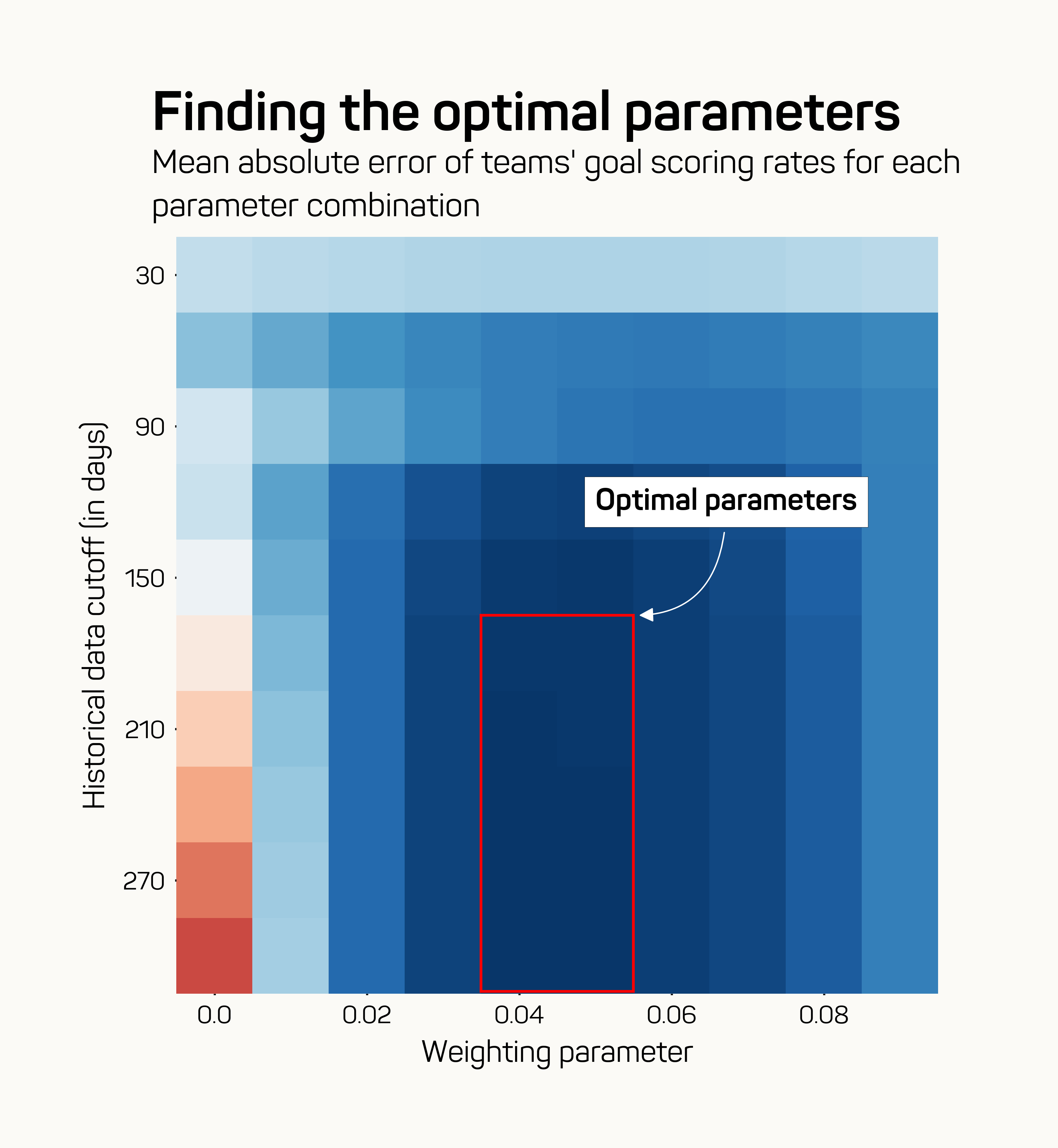
As you can see, using more than 180 days of data leads to diminishing returns. The optimal weighting parameter seems to be around 0.04. That means games further back than 180 days in the past only have a weighting of 0.1% or lower, making using data going back further mostly pointless. In the remainder of this blog, I’ll call the model we created here the bookie model.

As a comparison, I’ve also fitted a standard Dixon-Coles model on actual game outcomes. This model will be called the goals model benchmark. It is interesting to note that the optimal goals model includes data of up to 5 seasons back, compared to 180 days for the bookie model. This is a big pro for the method displayed in this blog, as it seems you don’t need much historical data to get started.

Results

Running the bookie model on the latest available data with the optimal parameters, you get these current team ratings for attack and defence. I decided to display the ratings as the expected goal scoring rates (for and against), against an average Premier League team, while playing at home.

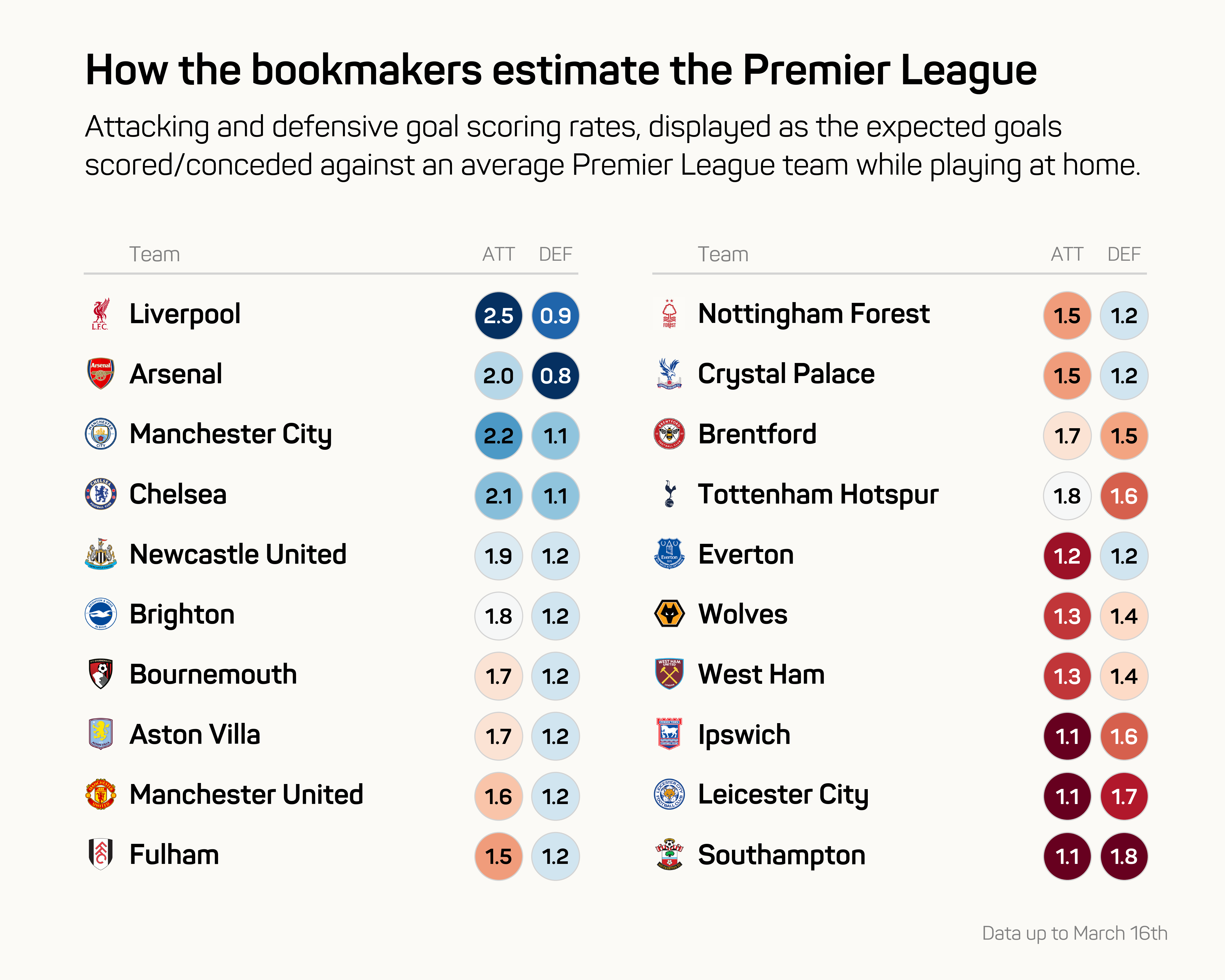
Interesting points for me were Nottingham Forest still being in the bottom half despite having the 5th best goal difference in the league thus far. Also, Spurs being 6th in attacking rating, but among the bottom 4 in defence. On the flip side of that is Everton, who are 4th worst in attack, but among the top half in defence.

Predicting future bookmaker odds

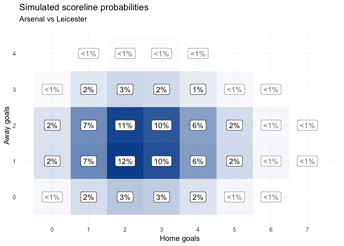
Now, we can use the fitted model to predict future games and bookmaker odds. To make the following section clearer, let me use an example. Let’s say at the beginning of March we wanted to predict Liverpool - Southampton. Here’s how a prediction could look like, vs. the actual bookmaker odds:

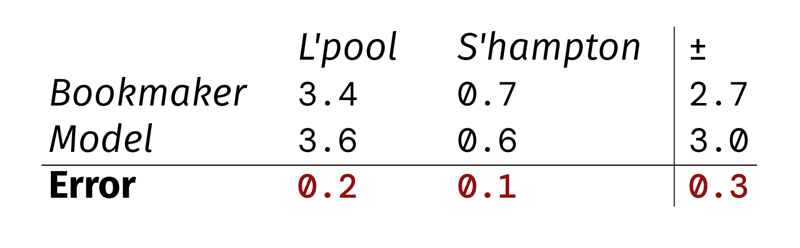
In this example the team level error is 0.15 on average. The goal difference error is 0.3.

To get the accuracy of this method over a large sample of games, I ran a backtest from the start of the 2015-16 season. Essentially, for every matchday we fit a model on all games that had happened until that point in time, looking back 180 days for the bookie model or 5 seasons for the goals model. Then, with the fitted model, we predict the next set of games. From this, it turns out the team level error for the bookie model is only 0.1 on average, and the goal difference error is only 0.16 on average. Compare that to the goals model benchmark, which has a team level error of 0.2 on average, and a goal difference error of 0.32. That’s 2 times worse on both metrics!

Here’s that visualised as a distribution of the team-level errors for both models:

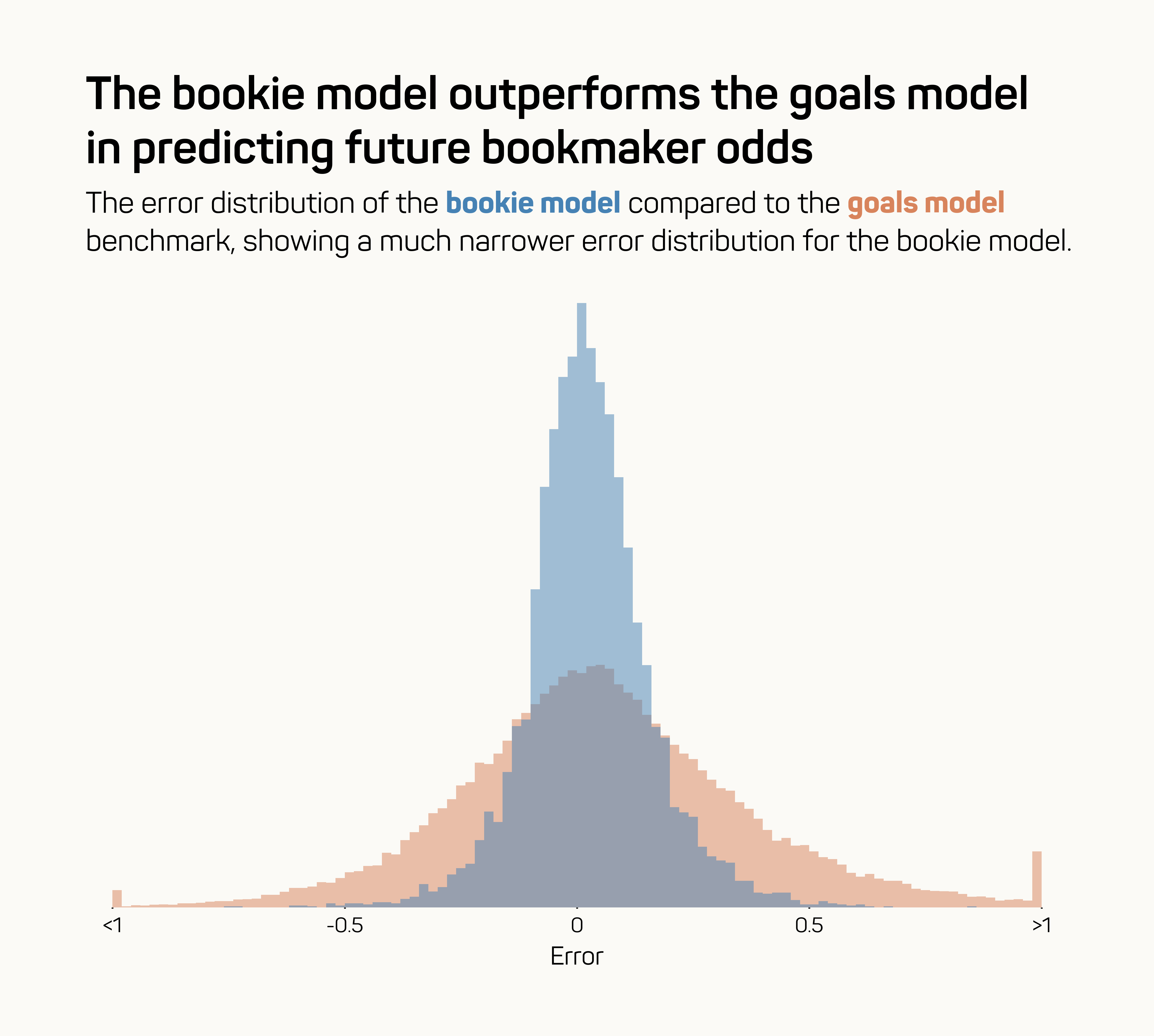
It’s clear that if you want to predict future bookmaker odds, using the bookie model leads to much better results than using the goals model benchmark.

A fair criticism here would be that we’re focussing too much on predicting future bookmaker odds, and not actual match outcomes. It would make sense that previous bookie odds highly correlate with future bookie odds, thus giving the bookie model an unfair advantage. To completely level the playing field, below I’ve compared both the bookie model, the goals model benchmark, and actual bookmaker opening/closing odds, based on how good they are at predicting the actual result — both in the near and in the distant future. For this we’ll be using the Ranked Probability Score (RPS) statistic, commonly used to assess the accuracy of results predictions.

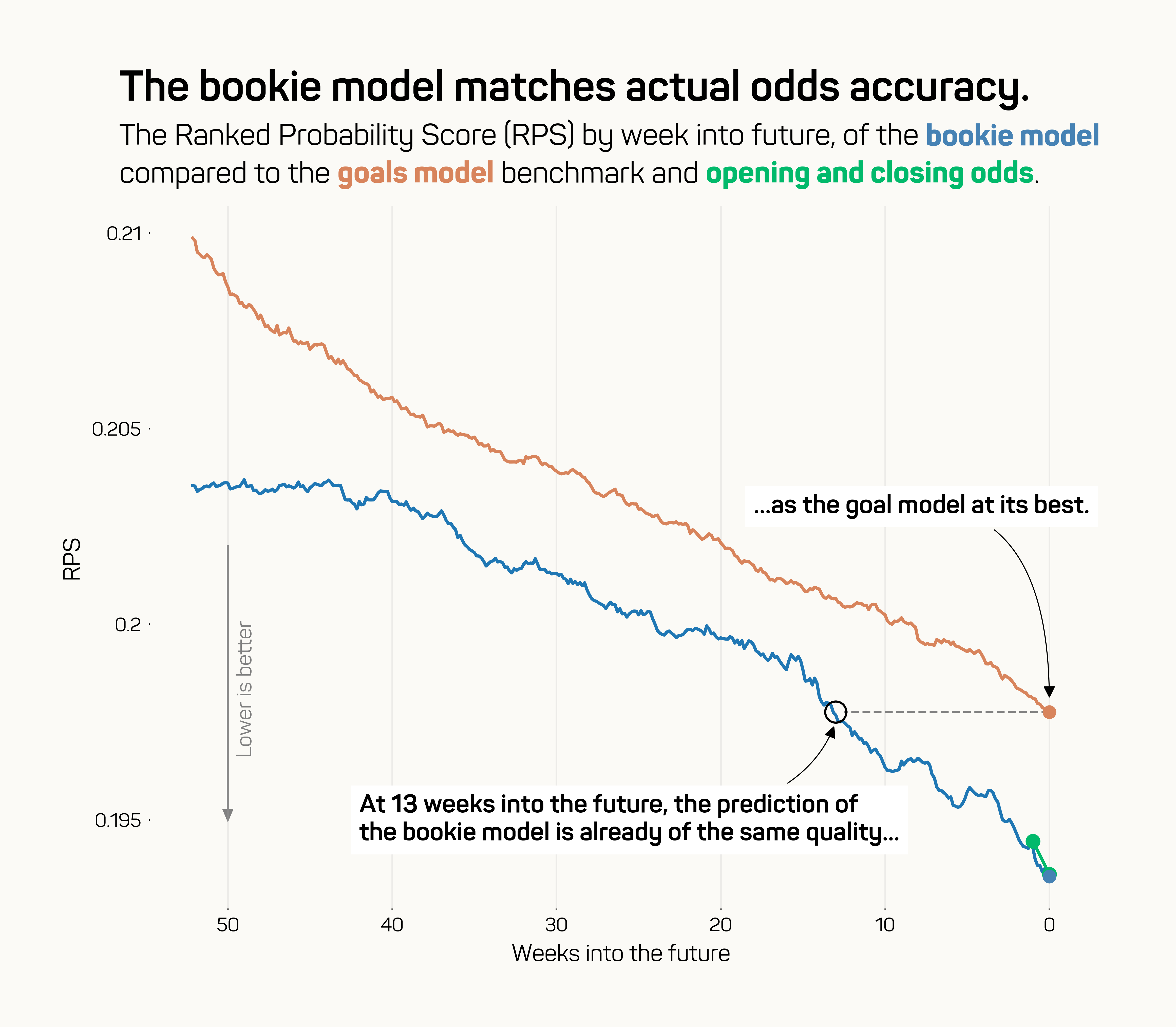
As you can see, the bookie model outperforms the goals model benchmark by a pretty wide margin. Even when predicting 12 weeks into the future, it’s still better than when the goal model predicts 1 day into the future. In other words, if we’re predicting, say, Liverpool - Southampton for a hypothetical game in July this season — the bookie model would be able to give you a better prediction today, then the goal model benchmark would be able to give you 1 day before the game, with 12 weeks of extra data.

Furthermore, when predicting in the week leading up to the game, the bookie model would give predictions of roughly the same accuracy as actual bookmaker odds.

Discussion

Interpretation

Instead of using goals or xG, the idea of this post is to use bookmaker odds instead. Doing this actually leads to a pretty interesting definition difference in what we are measuring:

• When using goals or xG, we are estimating team attack/defence strength based on actual results/events.
• When using bookmaker odds, we are letting go of any actual events, and instead estimating team attack/defence strength based on how good the bookmakers/market think they are.

This means that, theoretically, a team can lose 0-5, and have their estimated ratings go up — as long as the bookmakers/market have faith in their next performance.

Past relevant work

Using bookmaker odds to measure team strength is not a new concept. Ben Torvaney modeled team strength based on bookmaker odds in this blog from 2017. However, Ben modeled the overall team strength using an ordinal logistic regression, leading to a single number for each team instead of separate attacking and defensive rates.

Improvements

In this blog I used Over/Under and Asian Handicap odds. Using Correct Score odds directly makes even more sense, and might lead to better results. Unfortunately though, I don’t have (easy) access to these. On the flip side, you can use 1X2 odds as well, which are even easier to come across than what I used, though they might be less accurate.

The main other part that can be improved upon is how to handle the model around the start/end of a season. I noticed that the accuracy of the model is generally the lowest in August and May. In August, there will be promoted sides who have little to no recent data points to fit on. In May, some teams will be “on the beach” which could lead to big swings on how they are expected to perform.