
As you may or may not have noticed, in my latest blog I took a shot at quantifying how good our xG models currently are. Today I won’t look at overall performance, but I’ll go more in depth to see if the xG models have certain biases or not. Hopefully this will show where there is still improvement to be made, but also at which parts we’re already pretty good.
Just like last time, to know if the results we achieve are any good, we’ll have to know how they should be if the model were perfect. For this purpose I’ll use a simulation of a ‘perfect’ model (same as last time) as comparison. Basically what I did is I simulated the xG values from my own model to see what the connection between the xG values and actual outcomes should look like. For a more elaborate explanation please check this blog of mine. I will also be including a model that assigns all shots the same value of 0.095, the average conversion rate of a shot. In general we’ll expect any xG model to be better than that simple model, and we aim to approach the ‘perfect’ model.
Home/away bias
The first bias I’ll look at is the home/away biases. Basically what the test will look at is whether the xG models tend to over/underestimate to amount of goals scored in home/away games. What I did for this was simply look at the amount of xG each model assigned to home teams and compare it with how many goals were scored by home teams (similarly for away teams). This gave the following results:
| Goals/game | xG/game | |
| home | 1.26 | 1.30 (+0.04) |
| away | 1.05 | 1.08 (+0.03) |
The results are quite encouraging. In the 260 match sample I’m using the models slightly overestimated to numbers of goals that were actually scored, but the differences are minimal. The differences are so minimal that I’m pretty sure they can be called random variance.
The main point however is that the models over/underestimate home and away matches similarly. Individually the models were spread out a bit more, but none had a significant bias towards home or away teams.
Score bias
The other bias I’ll look at is score bias. What that means is that it’s possible some scores are over/under estimated by certain models. For instance, a model might systematically under predict the amount of xG for matches that have big scores like 5-0. On the other hand a model can over predict the amount of xG for matches that end in 0-0.
This will be quite interesting, as I often here people critique single match xG plots when the actual score and the xG score don’t align. People generally quickly start to question the model’s accuracy when the differences between what happened and what the plot says are big.
However, a fundamental thing to understand is that when a match ends in 1-1, we don’t expect the xG score to be 1.0-1.0 on average.
Wait what? Obviously if the xG score for a match is 1.0-1.0, in general the actual outcome we expect will also be 1-1. However the other way around this does not hold. This might seem weird, but it becomes clearer when we look at matches that end in 0-0. Would we expect the xG score to be 0.0-0.0 as well? No, of course not! The average match that ends in 0-0 will surely have had some chances, so the xG score must be larger than 0.0-0.0. Similarly this is true for matches that end in 1-1 or any other score.
So what xG scores do we expect? Simulations of the ‘perfect model’ gave the following plot:
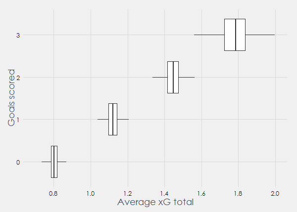
On the y-axis we can see the amount of goals scored by a team, and on the x-axis the average xG that such a team will have scored. The boxplots show 200 simulations of 260 games in the Premier League, and for each simulation the average xG score was taken when x goals were scored.
As we can read from the plot, when a team scores 0 goals in a game, on average we expect it to have about 0.8 xG. If a team scores once, it will have an average of about 1.1 xG. If a team scores twice it we expect it to have about 1.45 xG and when a team scores 3 times about 1.78 xG. The cause of this is that the underlying distribution of xG scores is not uniform. Obviously I don’t know the actual underlying distribution but my own model will serve as an approximation here. Let’s add the models and see how they perform:
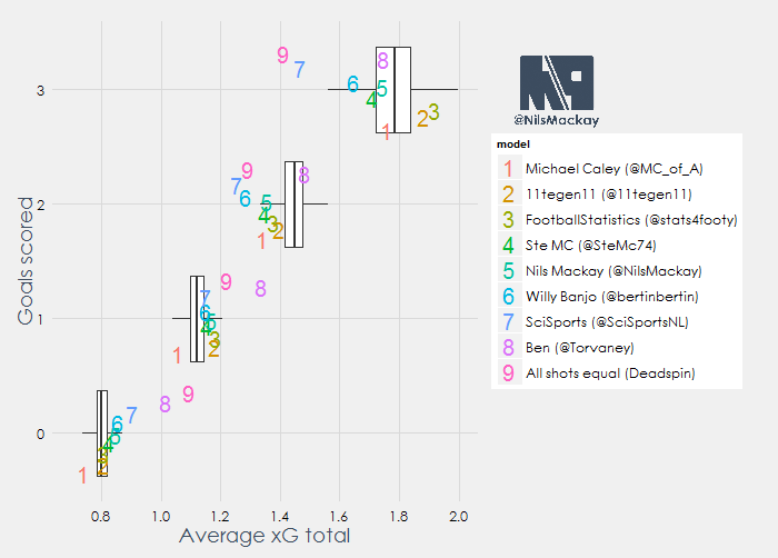
There’s a lot to see here so let’s start by explaining how this is displayed. On the right we can see the models that were evaluated in my latest blog, with the number corresponding to how they performed (1 is best, 9 is worst). In the plot each number is shown for each row once, and they are scattered a bit so the numbers don’t overlap.
In general what we can see here is that models 1 to 5 are within the area of the boxplot in all 4 cases. This means that the more accurate models also perform better in this bias test. Model 6, 7 and 8 are outside of the boxplot area once or more, whereas the naïve Deadspin model isn’t within the boxplot area a single time. In general what we can take from here is that the better models tend to have smaller biases (as expected), and that simple models might seem decent over large samples but they make consistent errors on smaller samples. One other thing I noticde is that when a team scores 1 goal, all models but one (Caley) overestimate the average amount of xG. Similarly, when a team scores 2 goals, all models but one (Torvaney) underestimate the average amount of xG. Whether this is due to the sample or a structural phenomenon I’m afraid I can’t tell for sure.
Concluding
Not all xG models are the same. When I see a statistic that uses xG I usually just assume it’s correct, while my analysis has shown that especially simpler models can make big systemic errors. I feel like the use of a too simple xG model might lead you to wrong conclusions. On the other hand half of the models I tested fall within the margin of error on every test I did. To me it seems like it is definitely worth it to invest a few extra hours to improve your xG model to get into that category. Simpler models can obviously still be used for analysis, but only if we understand their limitations and communicate this when publishing results.
Thus we come to the end of my 3-part piece on evaluating xG models. This was great fun so maybe it’s an idea to check back in a year or so to see how the state of xG models has changed. If you have any questions feel free to contact me on Twitter (@NilsMackay). If you want to read part 1 and 2: