
While browsing the web in March 2014 I stumbled over an article by Sander Ijtsma (@11tegen11) and Michiel de Hoog (@MichielDeHoog) explaining why Lex Immers, at the time a regular starter in the midfield of Feyenoord, was one of the best players in the Eredivisie. At the moment, that was a very controversial statement, as Immers was known to blow huge chances regularly. Many Feyenoord fans even blamed him for Feyenoord not winning the title that season, as Feyenoord finished second behind Ajax with only a four point difference. The general consensus was that Immers was not good enough for a team like Feyenoord.
The article however gave a different view of reality, as it introduced me to the concept of Expected Goals (xG), a measure which quantifies how big a chance is. Basically, every shot on goal is given a value between 0 and 1, illustrating the probability that the shot will end up in the back of the net. The article showed that Immers was actually not blowing chances at all, but was scoring as much as expected. Furthermore it showed that Immers was actually very good at creating chances for a midfielder as well. The more analytic way of looking at football resonated with me, probably also partly because I was at the time (and am currently) a student in Business Analytics. After reading the article I started following the football analytics community (mostly based on Twitter), very interested in what it had to offer.
Soon after, I decided I wanted to play around with the data myself, so I wouldn’t be dependent on answers of other people for my questions. My first step was to create my own xG-model. I have to admit it took longer than I expected at first, but the first version of it is now done. That is also what this article is about. I will explain my methodology, which is different from those of the models I’ve seen so far, and test to see if it is actually doing what it suggests: predicting the probability a certain shot will end up in the back of the net.
Methodology
The variables I used to predict the xG-values are the following:
- Shot location
- Whether it’s a header or a shot
- Whether it’s a penalty or not
- Whether it’s an own goal or not
Obviously there are many more factors which influence the chance of a shot going in, such as assist type, positioning of defenders and many more. Especially assist type is something I might pick up later, but for now I tried to keep it simple.
All models I know calculate the influence of shot location by dividing it into several factors such as distance to goal, and angle to goal (some use even more). Although it might be a good approximation, to me it sounded like a very complex way to compute the influence of location. The problem is that the goal posts make the distribution of values across the field very complex. For instance, a shot from 10 cm on the outside of the goalpost on the goal line will have an xG-value of practically zero, whereas the xG-value for a shot from 10 cm on the inside of the goalpost on the goal line will be about 1. This makes the exact values very hard to approximate by using angle and distance only.
To me it sounded more logical and precise to calculate the probability of a goal for a shot from a certain location by literally counting how many shots were taken from that exact position and counting how many of them ended up in the goal. Thus I divided the football pitch into squares of about a square meter, by making 100 squares in the length of the field and 50 squares in the width. Doing this for shots only gives the following field, in which a white corresponds with high xG-values and red with low xG-values:
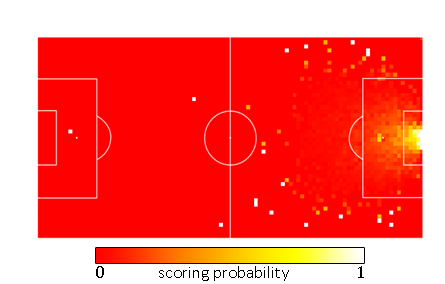
This is a mess. Even though I’ve used 10 seasons worth of shots (about 80,000 shots) for this, the sample size seems to be too small as the differences between neighboring squares is too big at certain locations. Furthermore, lucky long shots screw up the values for locations far from goal, as not many shots are attempted from such range. This makes the influence of one lucky goal very big on the resulting xG-value. The plot for headers was very similar.
To fix this, I decided to calculate the xG-value of a position by looking at all surrounding squares. This increases the sample size significantly, apart from the fact that it makes sense intuitively. The probability to score from a certain location won’t change significantly if you move less than 1 meter from that position. The actual shots from the square itself were given some extra weight.
This still has some issues. Lucky goals from long shots still have a huge influence on the xG-value for that square. Furthermore, by also counting the squares around the actual square, the problem with the goalposts arises again. To solve this, I decided that squares that didn’t have a minimum amount of shots taken from them and goals scored from them, would be set equal to the minimum xG-value, which is about 0.017. This means that no matter from where a shot is attempted it will always have at least an xG-value of 0.017. The idea behind this is that players will only attempt a shot if they think it’ll have at least a certain probability of ending up in the goal.
This sounds very specific, but really all it does is eliminate weird xG-values for squares with a too small sample size, and eliminate incorrect xG-values for squares from which there was never scored before. I think it’s safe to say that if in a sample of 80000 shots there isn’t a single goal scored from a certain location, the xG-value for that position is probably not that big.
The updated field, for shots only, then looks like this:
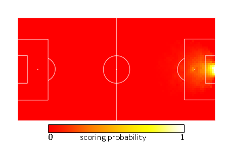
That looks better. You can clearly see that if the angle becomes too sharp, the chance to score drops immensely. The lucky long shots are accounted for, and the probability a shot becomes a goal rises quickly as you approach the goal. On the goal line it is nearly 100%. The field for headers is slightly different and generally gives lower values, but it looks quite similar.
Does it work though?
Although it looks pretty, the question that arises immediately is: does it work? Or in other words:
- Does it correlate well with the actual scoring chances within the sample data?
And more importantly:
- Is it able to predict the probability a shot outside the sample will end up in the goal?
Let’s start with the first one. To check if the model even agrees with the sample data, I grouped shots in small bins which are determined by xG-value. For example, if a shot is given an xG-value of 0.12 it is put in the bin that contains shots with values between 0.1 and 0.2. Next I calculated the average of the xG-values in the bin, and calculated the number of those shots that actually became a goal in real life. This gave the following table:
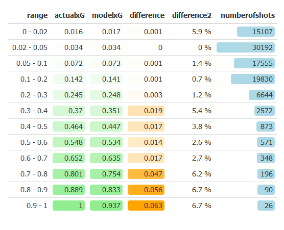
Just to clarify, the actualxG values are the percentages of shots within the bin that were scored. The modelxG is the average xG-value that the model assigned to those shots. Thus the values within the modelxG column are by definition within the range of the bin, which is not necessarily true for the values in the actualxG column.
Once again the effect of sample size is easily visible. The bins that contain the most of the shots have the highest accuracy. I’m pretty happy with the overall results. For most of the shots the actual bin value and the model bin value are less than 0.3% apart. For more rare shots this increases slightly, but the percentage differences for those shots is still fairly small. Notice that all 26 shots in the bin for values between 0.9 and 1 are scored thus far. This is likely a ‘hot streak’, as a 100% chance practically doesn’t exist. The model rates the average xG-value for those shots at around 94%.
The fact that the model’s values are close to the actual probabilities was to be expected. The model itself uses the number of times a shot went into the goal from that position. The fact that the values are similar doesn’t say that much, apart from the fact that the model describes its own sample adequately. More interesting is to see if the model is able to predict the chance a shot will become a goal for shots outside of the sample. The sample I used for this model are the seasons 12/13 and 13/14 for all 5 major leagues (Premier League (ENG), La Liga (ESP), Bundesliga (GER), Serie A (ITA) and Ligue 1 (FRA)). To see if the model has predictive value, I will do a similar test as above, except for the fact that the shots will be from the season 14/15 for those 5 leagues. These shots are not used to make the model. The table now looks as follows:
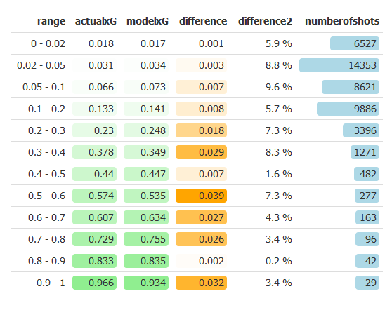
I’m very happy with the results. The difference for the small chances increased slightly, but is still below a 1% difference for most shots. As we can see the chances within the 0.9-1 bin are not all scored this time, as we expected.
Obviously these figures aren’t perfect. For instance, let’s look at the 0.1-0.2 bin. The model predicted the shots to be scored at around 14.1% of the time. If we would simulate all the 9886 shots within this bin using that probability, chances are about 1394 of them would be scored. In reality, only 1315 of those shots were scored. A simple binomial test shows us that if the probability of 14.1% is correct, the probability that 1315 or less goals would occur, is practically zero. That’s solid proof that the model isn’t perfect, but that’s also not the point of what I did. The model I created only uses location and some very basic things to calculate the scoring probability, while in real life the scoring probability is obviously dependent on more variables. It does however give a very decent estimate and is easy to understand. The addition of more variables should improve the results even more.
Hope you enjoyed! If you did, please share. My next blog will be expanding on this subject. It’s my first blog so any comments/advice/feedback would be appreciated. If you find a flaw in my reasoning or calculations please let me know!